
We analyse the average shape of binary search trees generated by sequences of random insertions and deletions. This is a classical problem in the theory of algorithms, in which a central concern is to ensure that the random trees generated within a particular scheme have low average height. Binary search trees have been used and studied by computer scientists since the 1950s. In 1962, Hibbard proposed a simple algorithm to dynamically delete an element from a binary tree [ Hibbard 1962 ]. Moreover, he also proved that a random deletion from a random tree, using his algorithm, leaves a random tree. Although the statement might seem self-evident, we will see shortly that this is not quite the case. More precisely, Hibbard’s theorem can be stated as follows: “If n + 1 items are inserted into an initially empty binary tree, in random order, and if one of those items (selected at random) is deleted, the probability that the resulting binary tree has a given shape is the same as the probability that this tree shape would be obtained by inserting n items into an initially empty tree, in random order.” Hibbard’s paper was remarkable in that it contained one of the first formal theorems about algorithms. Furthermore, the proof was not simple. Interestingly, for more than a decade it was subsequently believed that Hibbard’s theorem in fact proved that trees obtained through arbitrary sequences of random insertions and deletions are automatically random, i.e., have shapes whose distribution is the same as if the trees had been generated directly using random insertions only; see [ Hibbard 1962, Knuth 1973 ]. Quite surprisingly, it turns out that this intuition was wrong. In 1975, Knott showed that, although Hibbard’s theorem establishes that n + 1 random insertions followed by a deletion yield the same distribution on tree shapes as n insertions, we cannot conclude that a subsequent random insertion yields a tree whose shape has the same distribution as that obtained through n + 1 random insertions [ Knuth 1973 ]. As Jonassen and Knuth point out, this result came as a shock. In [ Knott 1975 ], they gave a careful counterexample (based on Knott’s work) using trees having size no greater than three. More precisely, they showed that three insertions, followed by a deletion and a subsequent insertion (all random) give rise to different tree shapes from those obtained by three random insertions. Despite the small sizes of the trees involved and the small number of random operations performed, their presentation showed that the analysis at this stage is already quite intricate. This suggests a possible reason as to why an erroneous belief was held for so long: carrying out even small-scale experiments on discrete distributions is inherently difficult and error-prone. For example, it would be virtually impossible to carry out by hand Jonassen and Knuth’s analysis for trees of size no greater than five (i.e., five insertions differ from five insertions followed by a deletion and then another insertion), and even if one used a computer it would be quite tricky to correctly set up a bespoke exhaustive search. Our goal here is to show that such analyses can be carried out almost effortlessly with apex. It suffices to write programs that implement the relevant operations and subsequently print the shape of the resultant tree, and then ask whether the programs are equivalent or not. As an example, we describe how to use apex to reproduce Jonassen and Knuth’s counterexample, i.e., three insertions differ from three insertions followed by a deletion and an insertion. Since apex does not at present support pointers, we represent binary trees of size n using arrays of size 2n − 1, following a standard encoding (see, e.g., [ Cormen et al 2001 ]): the left and right children of an i-indexed array entry are stored in the array at indices 2i + 1 and 2i + 2 respectively. It is then possible to write a short program that inserts three elements at random into a tree, then sequentially prints out the tree shape in breadth-first manner into a free identifier ch. The actual code is omitted here for lack of space, and can be found in [ Legay et al. ]. From this open program, apex generates the following probabilistic automaton:
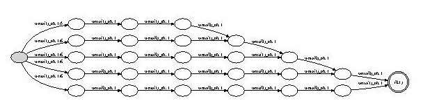
The upper path in this automaton, for example, represents the balanced three-element tree shape.

The probability that this shape occurs can be determined
by multiplying together the weights of the corresponding transitions, yielding a
value of 1 .
3
It is likewise straightforward to produce a program implementing three insertions
followed by a deletion and an insertion, all of them random—the code can
be found in [ Legay et al. ]. The corresponding probabilistic automaton
is the following:
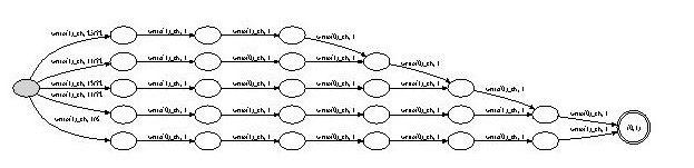
The reader will note that the balanced three-element tree shape occurs with
slightly greater probability: 25 . Thus the two programs are indeed not equivalent.
Note that none of this, of course, contradicts Hibbard’s theorem, to the effect
that the distribution on tree shapes upon performing two random insertions is
the same as that obtained from three random insertions followed by a random
deletion. The reason is that, although the distribution on tree shapes is the same,
that on trees is not. This is then witnessed by performing an additional random
insertion, which in the second case very slightly biases the resulting tree shape
towards balance, as compared to the first case.